


Further analysis of kinetic energy

Here we continue analysis of kinetic energy derived using our new method (RBN 2019/04). Firstly, the method should be verified to make sure it works reliably in all boat types and rowing styles. To do this, the data obtained with the BioRowTel system (n=12748) was retrospectively post-processed. The gain of the system kinetic energy dEk during the drive was calculated (velocities of the seat and the handle were averaged in crew boats) and compared with the sum of the measured work per stroke WpS in the crew.
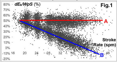
When data was plotted relative
to stroke rate (Fig.1), it appeared to split nearly equally into two trends: some
crews maintain nearly constant ratio dEk/WpS at all stroke
rates (A), but others decrease it at higher rates down to zero and even to
negative values (B).
To find out the reasons for this phenomena, we compared two male single scullers with distinctively different dEk/WpS ratios at racing stroke rates 33-34 spm (Table.1): Sculler 1 (1.93m, 95.0kg) had it at 55.6%, and sculler 2 (2.02m, 96.0kg) showed 6.3%.
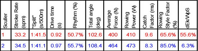
Sculler 2 had a significantly longer stroke, higher force and power, though both scullers had similar boat speed, but this could be an effect of weather conditions. As a result of having a longer stroke, sculler 2 had longer drive time and higher rhythm (ratio of the drive to the total time of the stroke cycle). Therefore, he had to move faster during the recovery, and both his handle (Fig.2,1) and seat (2) peak velocities were higher. To do this, he had to pull the stretcher harder and longer, so his boat acceleration during the recovery had a higher peak (3) and remained positive for longer (4): i.e. he starts pushing the stretcher closer to the catch. As a result, sculler 2 had a significantly higher boat velocity at the catch (5), and then it continuously decreased, as his boat acceleration had a later and deeper negative peak (6) which later became positive (7).
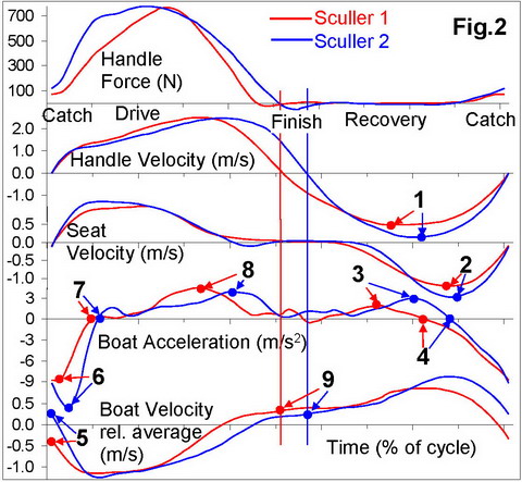
During the drive, sculler 2
had a later and lower positive peak of the boat acceleration (8), so at the
finish, his boat velocity was significantly lower than for sculler 1 (9),
nearly at the same level as it was at the catch. Therefore, the gain in boat
velocity and therefore kinetic energy was much smaller for sculler 2 than for
sculler 1. At higher rates 44-45 spm, the difference became even more dramatic:
dEk/WpS was 61.4% in sculler 1, and in sculler 2, it
was negative -16.4%, which means his boat velocity at the finish was lower than
at the catch.
Correlation analysis confirmed
the above findings: the timing and position of the negative peak of the boat
acceleration (Fig.2,6) had the most significant effect on the ratio dEk/WpS
(r=-0.59): the later the negative peak after the catch – the lower gain in
kinetic energy. The highest positive correlation (r=0.48) was found with timing
of the point 4 (Fig.2): the later the acceleration became negative before the catch
– the lower the gain in kinetic energy.
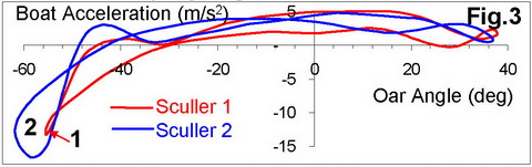
When the boat acceleration is plotted against oar angle (Fig.3), at the catch, sculler 1’s curve looks like a sharp edge, but for sculler 2, it has very large loop (2).
What does this all mean? Does
the lower gain in kinetic energy for sculler 2 mean that his technique is less
efficient? Or, does this only mean the new method doesn’t work properly for his
technique? The second option looks more trustworthy, because negative gains in
kinetic energy found in some crews at high rates are not possible: if the whole
system would not accelerated during the drive, it would slow down and
eventually stop, which doesn’t happen. Also, negative gain during the drive
would mean a positive gain of kinetic energy during recovery, which is
obviously incorrect. I would really appreciate your further ideas.
©2019 Dr. Valery Kleshnev www.biorow.com