BioRow data analysis

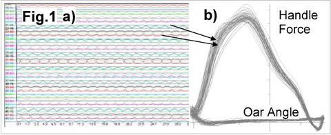
A common way to represent cyclic rowing data is plotting it as an X-Y chart, where the X coordinate is the oar angle, or handle position on a rowing machine. As an example, Fig.1,b shows the handle force curve in this way. Though this representation is more understandable and gives some impression about rowing technique, it is not useful for precise numerical evaluation, comparison and modelling of rowing biomechanics.

The key part of the BioRow data analysis is an algorithm of data averaging, which allows the conversion of information collected from an unlimited number of cycles into one typical stroke cycle. It was developed from 1991-93 (1) and was used for more than 25 years for data analysis both in a boat and on a rowing machine, as well as in other cyclic sports (canoeing and swimming). This method allows effective data analysis, storage and comparison, and very clear feedback and interpretation for rowers and coaches. Here it is explained in essence.

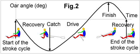
Firstly, the stroke cycle should be detected (Fig.2). For this, we use oar angle data (or handle position on a rowing machine) and define the start of the stroke cycle at the moment, when the angle crosses zero during the recovery (oars perpendicular to the boat axis, or the handle of a rowing machine passing over the knees). This point was chosen as it is the most idle period of the cycle, without sharp changes of the rower’s movement, where it is possible to pause naturally. Some other systems use the catch as the cycle start, which breaks apart this quick and very important phase of the stroke, and makes it difficult to analyse. Also, it is not natural to pause the stroke at the catch. In crew boats, the cycle is detected using only one oars data for the whole crew (usually, of the stroke rower, port side in sculling), which allows perfect synchronisation of the data.

The process of the data averaging starts with detecting the number of stroke cycles in a selected section of rowing, calculation of the average stroke rate SRav and its standard deviation SRsd. Then, the strokes are filtered and only the cycles within the range SRav±k*SRsd are used for averaging, where k=1 is usually chosen for strong filtering, 2 – for medium filtering and 3 – light filtering. The filtering is necessary because the high variation of the stroke rate makes typical patterns unreliable: it doesn’t make sense to average rowing at 20spm and at 40 spm.

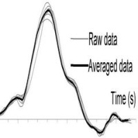
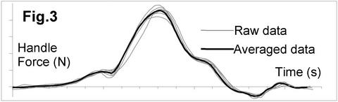
Cycles of various stroke rates have different numbers of data points: e.g., at a 25Hz sampling frequency, the cycle at 20 spm would have 75 data points, but at 44 spm – only 34 points, which makes such data difficult to handle. Therefore, arrays with a fixed number of points n are used for averaged data (n=50 was chosen). After filtering, these arrays are created for each data channel and time stamps Ti are assigned to each point, where Ti = (60/SRav)/n. For the raw data, the time from the beginning of the stroke cycle to each data point is different for various strokes (the cycle periods are still slightly different), which means it may belong to different phases of the cycle and should not be averaged. Therefore, raw data is interpolated to derive a value at the time Ti of each point of the averaged array, and then these values are averaged for all cycles in the sample. In other words, durations of raw cycles shrinks or stretches on X-axis to fit them to the duration of the average stroke cycle. Fig. 3 graphically represents the raw and averaged data for the handle force. Also, standard deviations could be derived for each point Ti, which allows evaluation of variability of rowing technique (RBN 2012/12).

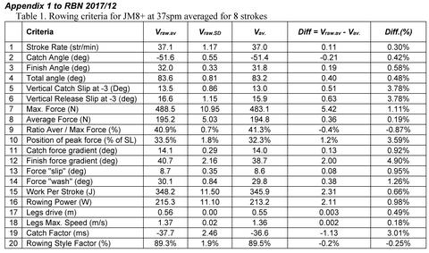
To check the validity of this method, various rowing criteria were derived for every stroke of the raw data (Vraw), then their averaged values (Vraw.av) were compared with the same criteria derived from the averaged arrays Vav (see Table 1 in the Appendix below). It was found that Vav values were slightly lower than Vraw.av, and for most criteria, the difference was within a range of 0.5%. It is important that for average force the difference was much smaller (0.19%) than for maximal force (1.11%), which could be explained by deviation of the timing of the peaks in each stroke, which makes the average curve smoother with lower peak, but insignificantly affects the area under the curve.

References

©2017 Dr. Valery Kleshnev www.biorow.com

References

1. Kleshnev V, 1996 Computer Technologies for Training in Cyclic Sports. In: Current Research in Sport Sciences, by V.Rogozkin & R.Maughan, Plenum Press, p.137-146